In this article, we'll discuss how we reduced inference latency by over 30% using a series of caches.

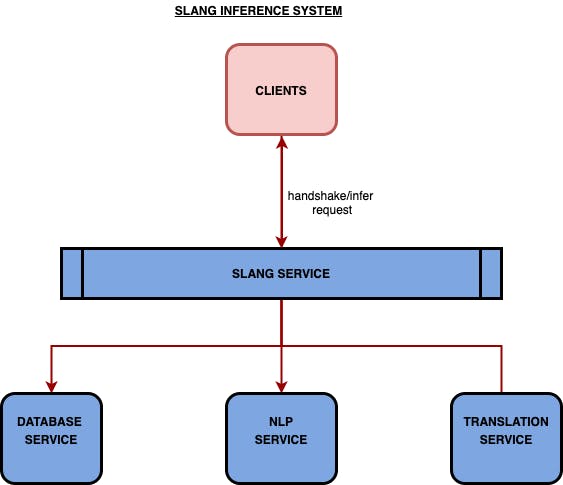
One of the significant services while building conversational technology like voice assistants is the infer service: the one responsible for handling the user voice queries and sending back the intent and entities recognized so that the app, in which the voice assistant is integrated, can perform the actions. Infer itself consists of 2 steps; the first is the handshake and then the actual inference request. The handshake consists of data such as prompts, hints, and other data that doesn’t change from inference to inference. As a result, the handshake does not need to precede every actual inference request. Still, it is required for one entire session of the app or when the user changes the language. Handshake enables the app to take actions based on the infer request.

However, an increasing number of incoming requests to the server can slow down the performance. We were trying to figure out a way to reduce this inference latency by a significant margin**.**

The high-level architecture:

Always look to your left and right before crossing the road:

When my team and I were building Slang CONVA, a multilingual voice assistant platform, we observed that each query latency that took a millisecond to respond increased to over 1 second for English and over 2 seconds for non-English. Before we dived into optimizing and making assumptions along the way, we started by understanding the overall system performance. Is the current response time the best we could do to handle infer requests or can we do better? What if we horizontally scale by adding more servers to handle the peak load? How would the system perform during average load and in peak? These were some of the questions that we initially set before we started investigating the performance bottlenecks.

As a standard process, best, average, and worst-case latency across multiple requests is measured by percentiles. You’d often see the words p50, p95, p99, etc. Different parameters are measured on these percentiles. p50 means the 50th percentile (meaning how well the system performs for 50% of the requests), p90 means the 90th percentile and so on for others.

‍

But why use percentiles?

Percentiles are better suited to measure latency metrics than averages. Consider this example; you have collected data on how long the user waits on your website to load. You have accumulated 6 data points (in milliseconds): 62, 920, 37, 20, 850, and 45. If you take the average load time, you get 322 ms. But 322 ms is not the accurate metric for the user experience. From this data, it’s clear some of your users are having a high-speed experience (less than 70ms), and some are having a prolonged experience (more significant than 850ms). But none of them has an average experience. Average can give you the incorrect metric.

The way to avoid being misled is to use percentiles. An excellent place to start is P50 and P90. To compute P50, just the median, sort the data points in ascending order: 20, 37, 45, 62, 850, 920. You get P50 by throwing out the bottom 50% of the points and looking at the first point that remains: 62ms. You get P90 by throwing out the bottom 90% of the points and looking at the first point, which remains: 920.

Investigation Step: Call Sherlock

To measure our current performance, we loaded the inference into a sandbox environment. We simulated load by sending a predefined number of actual requests at a predefined rate. We took into account the p75 latencies during high load.

Running tests under varying load and RPS (Request Per Second), we were able to identify three significant bottlenecks.

🙌🏻 Handshakes required sending the entire schema to the client for post inference operations, and doing so each time a client session ended was costly in terms of time and actual financial cost. The handshake schema could be huge for complex applications, and additional language support could increase in size to over 4MB. This was a bottleneck for the fast initialization of the application during launches.

🙌🏻 For every request, we made round trips to the NLP service, which is costly. It involves loading the model, extracting the intents and entities, and encoding and decoding the response.

🙌🏻 Our voice assistant platform is multilingual that supports regional Indian languages. However, under the hood, the NLP service works only in English, so the text requires additional translation and transliteration before being sent to the NLP. A request that involves the translation of the text can roughly take two times more time than an English text.

‍

The solution: it’s elementary, my dear Watson.

The answers to questions we initially set were found with the help of the test data. As it turned out, we were not efficiently utilizing our resources. There was much room for improvement with the current setup that we had.

If we closely analyzed the bottlenecks, we could see that most of the request time was spent on the NLP or the translation system. Most requests were repeated with a long tail of first-time requests. But, an NLP engine working on a model, until trained again, will reply with the same answer. Therefore, asking NLP to spend time on precisely the same request to get the same response is overkill. What if a layer could store a map between a given proposition and a given response. Every time the user says ‘onions,’ we look up the map and reply with the same response that the NLP engine had already processed. Imagine if hundreds of users speak the same set of sentences, the amount of processing time we would save.

The other obvious problem with the current system is the number of unnecessary calls the client has to make even when there are no schema changes.

‍

Can we do better here? Yes, we can!

⚡️ Preflight request:

A preflight request is a small request that the client sends before the actual client request. It is done to figure out if the more significant, more expensive request is even required. The larger request may not be necessary because the data backing it has not been invalidated yet. Thus we can use the same one the client had received on the previous request.

We used a preflight HEAD request first to check if the client’s handshake was needed. This gave us various improvements. The client did not have to do a handshake every time before an infer request since we implemented a client cache that gets invalidated based on preflight response.

⚡️ Cache All:

As we mentioned above, to improve the latency of NLP and translation responses, we decided to implement cache due to the nature of the response. The request did not have to go to the NLP or the translation each time; it could be reused across requests.

When designing a cache system in a multilayer system (layers such as client, server, model, among others), we could benefit from adding a cache to each layer in the design. Still, based on the nature of the layer, there were choices to be made on the type of cache and the invalidation strategy of the cache.

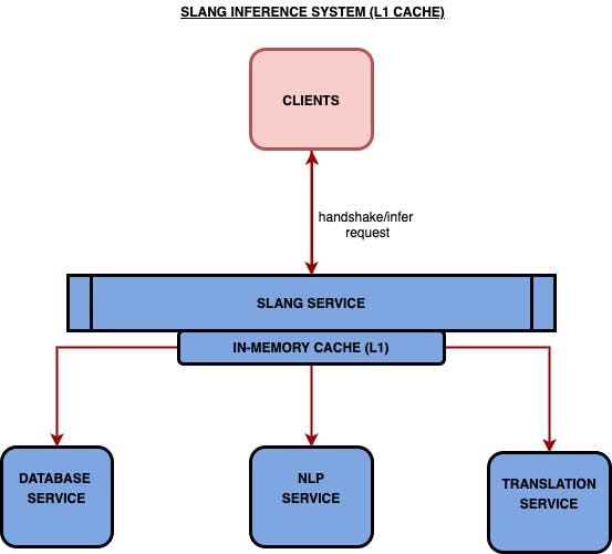
First was the L1 cache. An L1 cache is a volatile cache that stores data in RAM, which means that all the data is lost if you boot up the system again or the system crashes. But, the upside of an L1 cache is that they are the fastest of all the possible caches mentioned here. The volatile nature of the cache means that upon reboot, the cache has to be repopulated upon every inference request.

To account for the non-persistent nature of the in-memory cache, one can use an application like Redis or Memcached to create an L2 cache. This solves the problem by periodically saving the in-memory data into a hard disk. This reduces the impact of the volatility of an L1 cache.

We first implemented the L1 cache for resources in the critical path. The way it now works is when a handshake/infer request is fired, we do an in-memory cache lookup and fetch the result from the cache; however, if there is a cache miss, then the request goes all the way to NLP service and responses are saved in the in-memory cache so that subsequent request can retrieve the data from the cache.

We then started exploring Redis and Memcache. These are both in-memory data storage systems with support for data persistence. Redis is an open-source key-value store, and both store most of the data in memory. However, Redis supports operations on various data types, including strings, hash tables, and linked lists. And it was because of this rich feature support. We decided to go ahead with Redis for our L2 cache layer.

The Redis cluster is not self-hosted; instead, it is an instance hosted on the cloud provider. Cloud-hosted Redis ensures high availability and less overhead on the team to manage our cluster.

Two-level Cache System:

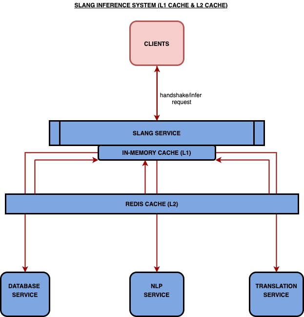
In the two-layer cache system design, imagine an inference request is sent to a Slang server. The response can be satisfied in one of the ways described below.

1. In the case of an L1 cache hit, the response is sent from L1.

2. In case of an L1 cache miss, we do an L2 cache lookup.

3. If the L2 cache is a hit, the response is sent from L2. On the way back, the L1 cache is warmed up with the response so that subsequent requests can be satisfied from the L1 cache.

4. If the L2 cache misses, the request is routed to the NLP Service.

5. On the way back, both L2 and L1 cache are warmed up with a response.

We have discussed the details of our multilayer cache system, but one thing is still missing. Let us understand when our cache evicts or invalidates the cache entry.

Eviction Policy :

Usually, the trade-off of a cache is that it is fast, and it will also be small. That means it will store fewer data in a smaller, faster, and more expensive memory unit. But that means, at some point, this memory will be filled up, and we need the policy to either ignore this for new requests or make space for the new request by removing old stored requests.

Our cache uses LRU (Least Recently Used) policy. LRU discards items that have not been used for a long time (more than other elements in the cache). The least recently used elements get evicted first when the cache gets full. It ensures that our memory doesn’t get bloated.

There are many possible eviction policies. But, to contrast, another possible eviction policy is Least Frequently Used. This means we order the requests from most used to least used and then remove the one that is used least with the logic that if not many people or processes need it, we can probably do without it. However, the problem here is that if we have a significant long tail of single-use requests, then almost 80% of the requests may be equivalent in that they are the least used. Then the cache will have a low hit ratio because as soon as the request is stored, it is removed for another one, and then that one has removed itself, and so on. This is called thrashing, and we implemented it.

Invalidation Strategy:

“There are only two hard things in Computer Science: cache invalidation and naming things” — Phil Karlton.

Another trade-off of a cache is that it will serve data faster, but it may not necessarily be the most recent data. Why is that so? Because the cache saves time by not looking into the database or performing some function that computes a possible new value for the data. This means we needed the policy to decide when the cache was stale and when we needed to recompute the data and refresh the cache possibly.

To invalidate the cache, we revisited our inference flow to understand better when the NLP/handshake/translation response would change. Schema changes required the retraining of the assistant. This means once the train is completed, all caches had to be invalidated. But how did we know if the train was completed? We could do that in two ways. The first was a broadcast system. Once the train had been completed, it would inform each of the train processes. The process then knew that on the subsequent inference, it should look at the database.

The alternative was, storing a flag in a particular position and having the concerned process continuously and periodically ping this flag. If the flag had changed, then that meant the underlying data or model had been invalidated, and the cache had to be refreshed on the subsequent inference. This was called the time-to-live (TTL) approach. Since the period (TTL) of the ping was configured into the service, the time until which it assumed the data was still ‘alive’ or fresh. Keeping a small TTL means that the cache very frequently invalidates its cache. If the TTL goes to 0, it is the same as not having a cache.

We used the second type. When an assistant got trained, it stored the timestamp at which the train completed the assistant’s metadata. Once the TTL ran out at inference time, it pinged the database for the assistant’s metadata. It looked at the last train timestamp. If it was more significant than the one it already knew, then that meant that a train had occurred since the last time. The process then invalidated its data and requested new data.

‍

Why do we need the layers? Why can’t one layer suffice?

Above, we spoke of two layers in the inference flow. There were many more caches that we implemented all over the server. Another one of these was the NLU model cache. The NLU model itself took about 2 seconds to load during inference. It first had to be fetched from the database, deserialized, and then be used. However, we could save time by caching the deserialized model itself. We did exactly that using the principles mentioned above; we cached the model itself and chose a TTL eviction strategy that evicted it based on the last timestamp available in the metadata.

So now we had a cache in the client itself, we had two different caches in the server which were keyed on the utterance, and we had an NLU model cache that was keyed on the assistant ID.

We had so many caches because they all had different trade-offs, and all saved processing time in different ways at their respective layers.

The client cache was only for that client. If a user spoke the same sentence on the phone, we could use a previous response keyed using the utterance, looking out for usual cache invalidation. But, since this cache was only for the client, the repetition of utterances did not benefit other clients since no data was shared across clients. This, of course, was the fastest from the client’s point of view since the request did not even reach the server, thus saving on network and processing time.

As mentioned at length above, the L1 cache saved time by not going to NLU to get the response since a previous response for the same utterance was stored and keyed by that utterance. However, the issue with this cache was that it was volatile and couldn’t keep its memory across reboots.

The L2 cache saved time by not having to go NLU but was slower than L1 and, of course, only worked if the utterance had been spoken before.

The final resort for all utterances was the actual NLU process if they were not present in the lower cache. But, if we knew for a fact that the assistant model had remained consistent with the one in the DB, why would we have had to look up the DB for a model every time?

So every layer had its purpose, and together, they maintained correctness and sped up returns due to the principle of locality. (Quick digression: What is the focus of locality, you ask? Ever used Instagram nowadays? You’ve seen one post with one thing, and then every post after that is the same thing?)

Looking at the explanation above, you may think that a better metaphor for caches is sieves, but hey, who doesn’t like themselves a piece of wedding cake!

Conclusion:

Some of the takeaways while solving the problem of inference latency:

1. Before diving into the problem — measure everything and work only with the data.

2. Prioritize what’s important vs. what you want. We prioritized dev time when implementing L1 over L2. But later, we found having a combination of 2 levels is the best approach for our performance.

3. Revisiting assumptions you made regarding how fast parts of your system works.

4. Understanding the request flow to understand the recurring patterns better.